
了解多少写多少吧
你长远一点的方向,希望是和地球大数据集成共享和挖掘利用相关的,例如如何制备AI-Ready的数据?有什么标准,有什么技术,结合什么样的场景?
AI-Ready程度(AI-Readiness)
美国国家海洋和大气管理局(NOAA)曾出版了一本《企业数据管理手册》,NOAA在本书中指出AI-Readiness包含以下要素:
数据质量
完整性
一致性
无偏性
时效性
来源和可靠性
访问
数据格式
交付选项
使用权(清晰、机器可读的许可证)
安全/隐私(保护受限数据)
文档
机器可读的元数据(关于数据的信息)
数据字典(关于每个参数的信息)
标识符(唯一标识数据集的编号/代码)
NOAA提出了一个四级成熟度模型,并详细描述了每个等级的特征,为数据集的AI-Readiness提供了一个快速评估的框架。
级别:0(Not AI-Ready)
- 数据一致性角度:未进行内部一致性的检查
- 数据访问角度:仅通过请求或订单系统对公众开放使用
- 元数据角度:没有数据字典可用,或数据字典不是机器可读格式(例如PDF)
级别:1(Minimal)
- 数据一致性角度:手动一致性检查
- 数据访问角度:只有一个非程序化的访问选项,例如文件下载
- 元数据角度:数据字典是机器可读格式(例如CSV、XML、JSON)
级别:2(Intermediate)
- 数据一致性角度:一致性检查部分自动化,部分结果有文档记录
- 数据访问角度:多种访问方式,且至少包括一个可编程访问方法(API)
- 元数据角度:数据字典使用机器可读的元数据标准
级别:3(Optimal)
- 数据一致性角度:完全自动化的内部一致性检查和报告;且考虑了与社区数据集的外部一致性
- 数据访问角度:除多种交付选项(下载、API)外,还有基于云和高性能计算提供的数据即服务(DaaS)
- 元数据角度:机器可读的元数据标准;参数与行业标准或其他机构数据集标准协调一致
大纲
1.引言(AI-ready整体与领域总结)
2.AI-ready建设现状(政府、企业、科研机构)
3.AI-ready具体领域建设分析
4.AI-ready具体领域平台建设实践
5.总结与展望
chatgpt AI-Ready 数据制备的关键技术
1. 数据预处理技术
- 重采样/重投影:将多源数据统一到一致分辨率与坐标系统;
- 插值/缺失值填补:使用时空插值(如Kriging、IDW、LSTM插补)填充数据缺失;
- 归一化/标准化:满足模型输入需求;
- 标签生成:结合专家知识或规则自动生成训练标签(如土地利用类型、生态系统分类);
2. 数据集成技术
- 多源融合:融合遥感影像(光学、雷达)、气象站、模型输出等;
- 数据对齐与配准:空间配准、时间对齐、多尺度统一;
- 知识驱动融合:结合本体、规则与知识图谱提升语义集成质量;
3. 数据共享与服务技术
- 云原生数据服务:如基于 AWS、GEE(Google Earth Engine)、Open Data Cube;
- API/OGC标准服务:WMS/WCS/WFS/CSW 等;
- 智能语义检索:结合知识图谱与语义标签进行智能查找;
AI-ready Snow Radar Echogram Dataset (SRED) for climate change monitoring
• Surface tracking and flattening: Figure 2(a) shows an example echogram prior to surface tracking and flattening. In its unprocessed state, the depth at which the surface (air-snow or air-ice boundary) appears varies depending on the surface relief and topographical changes across the surveyed terrain. This variability makes it challenging to accurately visualize and analyze the isochronous snow layers over long distances. To address this, the dataset echograms are transformed to represent a perfectly flat surface, which is essential for enhancing the visibility of stratigraphic snow layer boundaries and facilitating layer tracking algorithms. Surface tracking involves identifying the surface bin (range index) in each rangeline of the echogram. This requires an adaptive detection approach because the radar backscatter power and surface return signal exhibit variability across rangelines due to differences in terrain, radar incidence angle, and environmental conditions. We developed an adaptive surface detection algorithm based on the Constant False Alarm Rate (CFAR) principle, augmented with auxiliary data from Digital Elevation Models (DEMs) derived from radar altimetry. The CFAR algorithm dynamically adjusts the detection threshold for each rangeline, accounting for variations in noise and signal strength. By incorporating DEMs, the algorithm further refines surface tracking by leveraging additional topographical context. After surface tracking, the surface bins are aligned across the echogram using a surface bin alignment algorithm. This step shifts each rangeline’s surface bin to a consistent index, effectively flattening the echogram. The result is an image where the surface appears perfectly flat, significantly improving the interpretability of snow layer boundaries. Surface flattening is a critical pre-processing step that facilitates subsequent operations, including along-track filtering and contrast enhancement.
• Detrending and 2D filtering: Due to propagation loss and media attenuation of the transmitted signal as it traverses the ice sheet, returns from deeper snow layers often experience significant signal-to-noise ratio (SNR) degradation. This can make it challenging to detect and track these deeper layers, as their weak signals are buried in noise. To address this, we apply custom detrending methods to enhance the visibility of deeper snow layers by compensating for signal attenuation and remove the power loss as a function of depth trend. This is done by fitting a third-order polynomial to the rangeline’s log-power data to remove the trend. The echogram creation process as detailed [30] already include coherent and incoherent integration to improve data SNR, however, to further improve the tracking performance of the deep learning models, additional mild along-track filtering is applied to the dataset’s echogram images. The volumetric backscatter from a snow resolution cell in S-band and C-band frequencies is typically a random process, which introduces stochastic fluctuations in the signal. When this randomness is pronounced, it leads to diffused pixels at the boundaries of snow layers, blurring the layer boundaries and complicating the task of layer detection. These blurred boundaries hinder the ability of deep learning algorithms to distinguish between layers accurately. To mitigate this issue, we apply loworder moving average filters in both dimensions in the linear power domain designed to smooth the data and enhance the contrast between adjacent snow layers, allowing for more precise layer tracking.
• Normalization: Finally, we normalized the pixel values in the echograms to the [0,1] range using a simple linear mapping from backscatter power (in dB) to echogram pixels to ensure quick deep learning model optimization convergence.
AI4Boundaries: an open AI-ready dataset to map field boundaries with Sentinel-2 and aerial photography
This section describes how the monthly cloud-free Sentinel2 surface reflectance composites for March to August 2019 (thus 6 months of four bands: R, G, B, NIR) were produced. Figure 5 provides an example of the dataset. The Sentinel-2 level-2A surface reflectance (SR) were derived from the Sentinel-2 level-1C top of atmosphere (TOA) reflectance data processed using the Sen2Cor processor (Main-Knorn et al., 2017) from the ESA SNAP toolbox (European Space Agency, 2023). The four spectral bands that are available at a spatial resolution of 10 m were selected (B2, B3, B4, and B8). The Scene Classification Layer (SCL) obtained from Sen2Cor was added as an extra band. Sentinel-2 processing was performed on the BDAP (Soille et al., 2018) using the open-source pyjeo (Kempeneers et al., 2019) Python package. Data cubes, consisting of merging all 2019 acquisitions for all 4 × 4 km2 chips, were created. The data cubes were extended with the acquisitions of the preceding (December 2018) and successive (January 2020) months. The extra observations served to mitigate the boundary effects at the beginning and end of the time series while applying temporal operations. These months were removed after the filter was applied. Only pixels identified as dark (SCL = 2), vegetated (SCL = 4), not-vegetated (SCL = 5), water (SCL = 6), and unclassified (SCL = 7) were considered as “clear”. In addition, outliers were detected using the Hampel identifier (Hampel, 1974), based on the pixel values in the red (B4) and near-infrared (B8) bands. The SCL was resampled to 10 m based on the nearest neighbour to obtain a regular gridded data cube. The Hampel filter calculates the median and the standard deviation in a moving window, expressed as the median absolute deviation (MAD). For the moving window, a width of 40 d was considered. Pixels below 2 and above 3 standard deviations from the median were identified as outliers for the NIR and the red bands, respectively. The respective values of 2 and 3 standard deviations for the lower and upper bounds were selected ad hoc based on a visual inspection of the results. The outliers in the red and NIR band domains were used to identify omitted clouds and omitted cloud shadows, respectively. The masked pixels from the SCL and the detected outliers were removed from the time series and replaced by a linearly interpolated time series using “clear” observations; in case of outliers near the beginning and end of the time series, values were extrapolated to the nearest “clear” observation. The resulting time series’ were then resampled to obtain gap-filled data cubes by taking the mean of the filtered and interpolated values every 5 d. Despite the SCL masking and the outlier detection, the resulting time series’ were still noisy. This is due to residual of atmospheric correction and non-accounted bidirectional reflectance distribution function (BRDF) effects. A subsequent smoothing filter was therefore applied, the recursive Savitzky–Golay filter (Chen et al., 2004). The original implementation has been developed for Normalised Difference Vegetation Index (NDVI) time series. It was adapted in this study to smooth surface reflectance values. A total of 15 observations at 5 d temporal resolution were used for the smoothing window size: 7 leftward (past) and 7 rightward (future) observations. The order of the smoothing polynomial was set to 2.
10.22
Data Readiness for AI: A 360-Degree Survey, ACM Computing Surveys, Vol.57 Issue 9, Article 219 (2025).
“Making data AI-ready: From FAIR to actionable intelligence” — Patterns (Cell Press), 2024
“FAIRness and beyond: preparing scientific data for AI applications” — Nature Scientific Data, 2024
“FAIR for AI: An interdisciplinary and international perspective” — Scientific Data / Nature commentary (2023).
参考
[1]钱力,刘志博,胡懋地,等.AI就绪的科技情报数据资源建设模式研究[J].农业图书情报学报,2024,36(03):32-45.DOI:10.13998/j.cnki.issn1002-1248.24-0173.
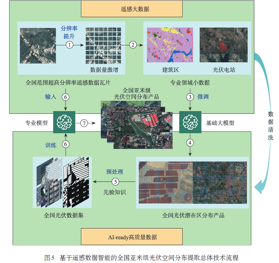
[1]何国金,刘慧婵,杨瑞清,张兆明,薛远,安诗豪,袁铭若,王桂周,龙腾飞,彭燕,尹然宇.遥感数据智能:进展与思考[J].地球信息科学学报,2025,27(2):273-284
Ibikunle 等 - 2025 - AI-ready Snow Radar Echogram Dataset (SRED) for climate change monitoring
d’Andrimont 等 - 2023 - AI4Boundaries an open AI-ready dataset to map field boundaries with Sentinel-2 and aerial photograp
Is your data ready for AI? https://www.youtube.com/watch?v=0Ec0tgdpDEU
美国国家科学基金会如何定义AI-Ready数据集 https://nadc.china-vo.org/article/20241219164120